A Deeper Dive into Linear Regression: Understanding, Application, and a Real-World Example

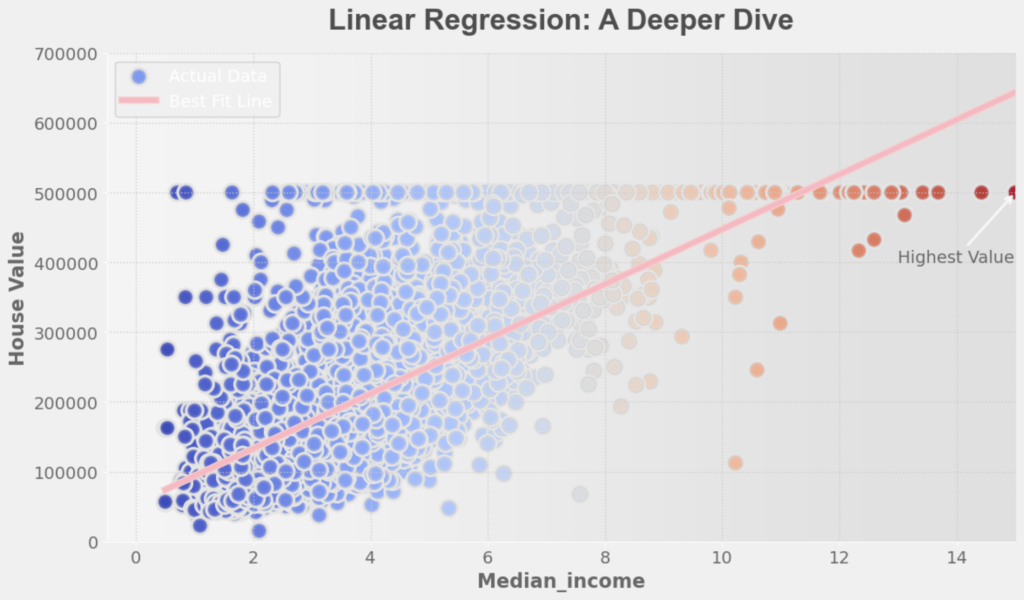
Linear Regression is a core technique in data science. While most of us learn the basics of linear Regression early on, fully understanding how and why it works allows us to apply it more effectively. In this blog, we’ll break down the core concepts, explain when and why to use them, and provide an end-to-end real-world example using housing prices.

What is Linear Regression?

Linear Regression is a method for modeling relationships between a dependent variable (the thing we are predicting) and independent variables (the things that affect the dependent variable). It works under the assumption that the relationship is linear – meaning a straight-line relationship exists between them.

Formula Breakdown

For simple linear Regression, the equation is:

Where:

For multiple linear Regression:

This means that we can use several independent variables to predict the outcome, not just one.

When and why should you use Linear Regression?

You should use linear Regression when your data shows a linear relationship between the independent and dependent variables. It’s simple, easy to interpret, and fast. However, it works best under certain conditions. These conditions are:

1. Linearity: The relationship between the dependent and independent variables should be linear.
2. Homoscedasticity: Residuals (prediction errors) should have constant variance. In simpler terms, the spread (variance) of the residuals should be roughly the same across all levels of the independent variables. Still confused? Read more on Homoscedasticity here:
3. Independence: Observation must be independent
4. Normality of Residuals: Residuals should follow a normal distribution

What are Residuals?

Residuals are the differences between the actual values (from the dataset) and the predicted values (from the linear regression model). Ideally, the residuals should be small and randomly distributed.

For example, if you’re predicting house prices:

• The actual price of a house is $300,000.

• The predicted price from the model is $290,000
• The residual (error) is $10,000

What is Constant Variance? also known as Homoscedasticity.

In linear Regression, we assume that the residuals have constant variance across all levels of independent variables. This means that the amount of error (or noise) in the predictions should be roughly the same, regardless of whether you’re predicting small or large values.

If this assumption holds, the residuals should not display any clear pattern and should be scattered randomly across a horizontal line when plotted.

Example:

Let’s say you are using linear Regression to predict house prices based on square footage. If the residuals have constant variance, they would like this when plotted against the independent variable (square footage):

#importing the required libraries
import numpy as np
import matplotlib.pyplot as plt
from sklearn.linear_model import LinearRegression
from sklearn.datasets import make_regression

#Generate a simple linear regression dataset
X, y = make_regression(n_samples=100, n_features = 1, noise=10, random_state=42)
model = LinearRegression()
model.fit(X,y)
y_pred = model.predict(X)

#Calculate residuals
residuals = y - y_pred

#Plot residuals
plt.scatter(X, residuals)
plt.axhline(y=0, color='r', linestyle='--')
plt.title("Homoscedasticity (Constant Variance)")
plt.xlabel("Independent Variable (X)")
plt.ylabel("Residuals (y - y_pred)")
plt.show()

In this plot, the residuals are scattered randomly and evenly across the range of the independent variable (X – square footage), indicating Homoscedasticity (constant variance). The residuals don’t become larger or smaller as the size of the house increases.

What happens When Variance is Not Constant (Heteroscedasticity)?

If the variance of the residuals changes as the independent variables increase or decrease, this is called heteroscedasticity, and it violates one of the key assumptions of linear Regression.

Here is what a plot might look like if the residuals exhibit heteroscedasticity:

#Create a dataset where variance increases with X (heteroscedasticity)
X_hetero = np.random.rand(100,1) * 100
y_hetero = 2 * X_hetero.ravel() + np.random.randn(100) * (X_hetero.ravel()) #increasing noise with X

#Fit the model
model_hetero = LinearRegression()
model_hetero.fit(X_hetero, y_hetero)
y_pred_hetero = model_hetero.predict(X_hetero)

# Calculate residuals
residuals_hetero = y_hetero - y_pred_hetero

# Plot residuals
plt.scatter(X_hetero, residuals_hetero)
plt.axhline(y=0, color='r', linestyle='--')
plt.title("Heteroscedasticity (Changing Variance)")
plt.xlabel("Independent Variable (X)")
plt.ylabel("Residuals (y - y_pred)")
plt.show()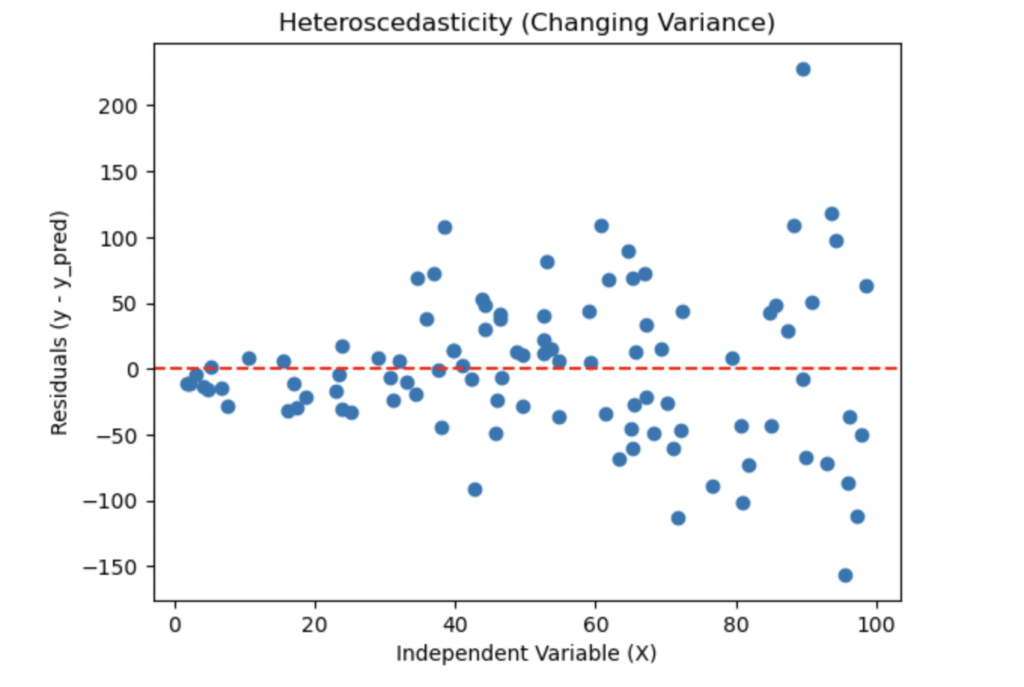

In this plot, you can see that as the independent variable (X – square footage of the houses) increases, the spread of the residuals also increases. The errors for larger houses are much more spread out than for smaller houses. This suggests that the model might be underestimating the price for smaller homes and overestimating the price for larger ones.

Why is Homoscedasticity Important?

When the variance of residuals is not constant (heteroscedasticity), it can lead to problems:

• Biased standard errors: This can lead to incorrect conclusions in hypothesis testing, making your model less reliable.
• Inaccurate predictions: The model might perform well for some values but poorly for others.

If heteroscedasticity is detected, you may need to use a different model( e.g., generalized least squares) or transform the data to correct it.

When to avoid Linear Regression:

If your data doesn’t meet these assumptions, linear Regression may produce biased results. For example, it won’t work well with non-linear relationships, outliers, or when the independent variables are highly correlated with each other, which is also known as multicollinearity.

Real-World Example: Predicting House Prices Using Linear Regression

Let’s walk through a real-world example to make this clearer. We will use a house price dataset I retrieved from https://www.kaggle.com/datasets/shibumohapatra/house-price called California house price. This example will give you an end-to-end data science process.

Step 1: Loading and Understanding the Dataset

First, let’s start by loading the housing dataset. This dataset includes various features like square footage, the number of bedrooms, the proximity to the ocean, and much more, which we will use to predict house prices.

#importing necessary libraries
import pandas as pd

#load the dataset
file_path = 'Dataset/1553768847-housing.csv'
df = pd.read_csv(file_path)

#Take a look at the first few rows of the dataset
df.head()

Dataset Overview:

• Longitude: Geographical longitude.
• Latitude: Geographical latitude.
• Housing median age: The median age of the housing in the area.
• Total rooms: The total number of rooms in the house.
• Total bedrooms: The total number of bedrooms in the house.
• Population: The number of households in the area.
• Median Income: The median income of residents in the area
• Ocean proximity: Proximity of the house to the ocean (categorical).
• Median house value: The target variable (house price).

Now that we understand the data, let’s move to preprocessing.

Step 2: Data Preprocessing

Before feeding the data into our linear regression model, we need to clean it and transform it into a usable format. This involves:

• Handling missing values (if there are any)
• Encoding categorical variables (All data that is categorical need to be transformed into a value that linear Regression can understand).
• Scaling numerical features.

#Check for missing values
print(df.isnull().sum())

#Drop rows with missing values for simplicity
df_cleaned = df.dropna()

#One-hot encode the categorical variable 'ocean_proximity'
df_encoded = pd.get_dummies(df_cleaned, columns = ['ocean_proximity'], drop_first=True)

#Inspect the dataset after preprocessing
df_encoded.head()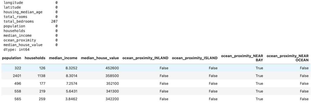

Explanation:

• We dropped rows with missing values. In our case, total_bedrooms has 207 missing values.
• We applied one-hot encoding to convert the categorical variable ocean_proximity into a format that can be used in linear Regression.

Step 3: Splitting the Data

We’ll now split the dataset into two parts:

• Training data (80%): Used to train the model.
• Test data (20%): Used to evaluate the model’s performance.

from sklearn.model_selection import train_test_split

#Define the features (independent variables) and taget (dependent variable)
X = df_encoded[['longitude', 'latitude', 'housing_median_age', 'total_rooms', 
                'total_bedrooms', 'population', 'households', 'median_income'] +
                list(df_encoded.columns[df_encoded.columns.str.contains('ocean_proximity')])]
# Ensure numeric data types and handle invalid values
X_numeric = X.apply(pd.to_numeric, errors='coerce')

# Impute missing values using the mean of each column
imputer = SimpleImputer(missing_values=np.nan, strategy='mean')
X_imputed = imputer.fit_transform(X_numeric)

# Convert back to DataFrame (for ease of use later)
X_imputed = pd.DataFrame(X_imputed, columns=X_numeric.columns)

# Replace infinite values, if any, with NaNs and then fill them
X_imputed.replace([np.inf, -np.inf], np.nan, inplace=True)
X_imputed.fillna(method='bfill', inplace=True)  # Back-fill strategy for imputation

y = df_encoded['median_house_value']

#Split the data into training and testing sets
X_train, X_test, y_train, y_test = train_test_split(X_imputed, y, test_size = 0.2, random_state=42)

Explanation:

• We selected the relevant features (independent variables) and defined our target variable (median_house_value).
• We split the data into a training set (80%) and a test set (20%)

Step 4: Checking all the assumptions

Remember, before diving into linear Regression, checking whether the data meets the assumptions required for linear Regression to work effectively is crucial. These assumptions include:

• Linearity: There should be a linear relationship between the independent and dependent variables.
• Homoscedasticity: The variance of residuals should be constant (no heteroscedasticity).
• Multicollinearity: The independent variables should not be highly correlated with each other.
• Normality of Residuals: The residuals should follow a normal distribution.
• Independence of Residuals: The residuals should be independent (e.g., no autocorrelation).

Let’s break these down one by one and check each assumption with the dataset.

Checking Linearity

The relationship between each independent variable and the target variable (house price) should be linear. We can visualize this using scatter plots.

import matplotlib.pyplot as plt
import seaborn as sns

#Plot scatter plots for key features against the target variable
features = ['longitude', 'latitude', 'housing_median_age', 'total_rooms', 'total_bedrooms', 'population', 'households', 'median_income']
for feature in features:
plt.figure(figsize=(6,4))
sns.scatterplot(data=df_encoded, x=feature, y='median_house_value')
plt.title(f'Scatter plot of {feature} vs. House Price')
plt.show()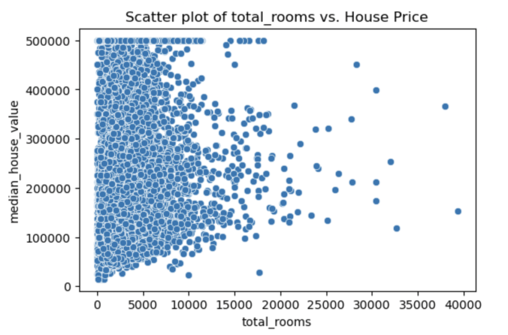

Explanation:

As you can see, the scatter plot shows the relationship between the total number of rooms and the house price, showing a trend where, as the number of rooms increases, the house price also increases. However, the relationship does not appear to be linear, and there is a considerable spread in house prices for homes with similar room counts. This spread suggests potential variability influenced by other factors not captured simply by the number of rooms.

None of the other independent variables seems to be linear with the dependent variable. Usually, in a case like this, you can consider using different algorithms because linear Regression will not be as effective as we would want it to be. For the sake of the blog, I will continue to use linear Regression.

Checking for Homoscedasticity (Constant Variance of Residuals)

We need to ensure that the variance of the residuals is constant. This can be checked with a residual plot.

from sklearn.linear_model import LinearRegression
model = LinearRegression()
model.fit(X_train, y_train)

# Get the residuals (difference between actual and predicted values)
y_pred = model.predict(X_train)
residuals = y_train - y_pred

# Plot residuals to check for homoscedasticity
plt.figure(figsize=(6, 4))
sns.scatterplot(x=y_pred, y=residuals)
plt.axhline(0, color='r', linestyle='--')
plt.title("Residuals vs. Predicted Values")
plt.xlabel("Predicted House Prices")
plt.ylabel("Residuals")
plt.show()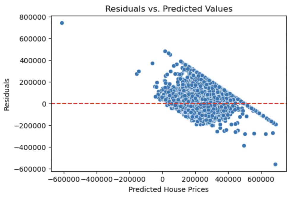

Looking at the plot, we see signs of heteroscedasticity (Changing Variance). The variance is not constant, again showing that linear regression is not reliable in this case.

Checking for Multicollinearity

Multicollinearity occurs when two or more independent variables are highly correlated with each other, which can negatively impact the model. We check for multicollinearity using the Variance Inflation Factor (VIF).

# Calculate VIF for each feature
vif_data = pd.DataFrame()
vif_data["Feature"] = X_imputed.columns
vif_data["VIF"] = [variance_inflation_factor(X_imputed.values, i) for i in range(X_imputed.shape[1])]

print(vif_data)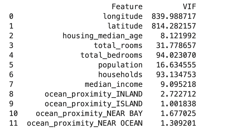

Explanation:

• VIF value close to 1: Little correlation
• VIF between 1 and 5: Moderate correlation
• VIF greater than 5: Strong correlation, potential multicollinearity

In our case, we should consider removing features with a VIF higher than five because these are major signs of multicollinearity.

Checking Normality of Residuals

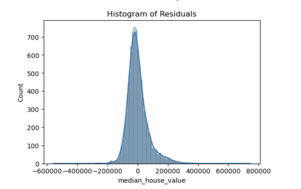
The residuals (errors) should be normally distributed. We can check this assumption using a Q-Q plot and a histogram of residuals.

import scipy.stats as stats

# Q-Q plot for normality of residuals
plt.figure(figsize=(6, 4))
stats.probplot(residuals, dist="norm", plot=plt)
plt.title("Q-Q Plot of Residuals")
plt.show()

# Histogram of residuals
plt.figure(figsize=(6, 4))
sns.histplot(residuals, kde=True)
plt.title("Histogram of Residuals")
plt.show()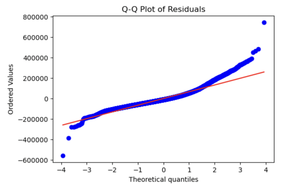

Checking for Independence of Residuals (No Autocorrelation)

Q-Q Plot Analysis:

• The Q-Q plot shows that the residuals deviate from the straight line, especially in the tails (both left and right). The extreme residuals indicate that the distribution of residuals is skewed or heavy-tailed, suggesting that the normality assumption might not be fully satisfied.

Histogram of residuals Analysis:

• The histogram of residuals looks somewhat bell-shaped, but there are some deviations. Specifically, the distribution appears to be slightly skewed, with a long tail on the right side. This again suggests that the residuals are not perfectly normally distributed, with some potential outliers or high errors.

Checking for Independence of Residuals (No autocorrelation)

We can use the Durbin-Watson test to ensure that the residuals are independent. This test checks for autocorrelation (correlation between residuals).

from statsmodels.stats.stattools import durbin_watson

# Durbin-Watson test for autocorrelation of residuals
durbin_watson_test = durbin_watson(residuals)
print(f"Durbin-Watson Test: {durbin_watson_test}")

Interpretation:

• A Durbin-Watson value of 2 indicates no autocorrelation in the residuals.
• Vales between 1.5 and 2.5 are generally acceptable, implying that there is little to no autocorrelation in the residuals.

Since our result is very close to 2, we can conclude that the residuals in our linear regression model are independent, meaning there is no significant autocorrelation.

We have checked all assumptions for our linear regression model. Out of all the assumptions, we only pass one: “Checking for the independence of residuals.” Usually, failing one assumption would call for us to use another algorithm or try to fix our data so that the chosen algorithm can be effective. But for the sake of this blog and learning, let us proceed with Linear Regression to interpret the results.

Step 5: Building the Linear Regression

With the data cleaned and split, it’s time to build and train the linear regression model using scikit-learn’s LinearRegression class. We previously did this in our “Checking for Homoscedasticity (Constant Variance of Residuals)” step, but It does not hurt to do it again.

from sklearn.linear_model import LinearRegression
model = LinearRegression()
model.fit(X_train, y_train)

• We created an instance of the LinearRegression class and trained it using the fit() method with the training data (X_train and y_train).
• The model will now “learn” the relationships between the features and the house prices from the training data.

Step 6: Making Predictions

Now that the model has been trained, we can use it to make predictions on the test set (unseen data).

# Make predictions on the test set
y_pred = model.predict(X_test)

• We used the predict() function to generate predictions for the test set. These predictions will be compared to the actual house prices to evaluate the model’s performance.

Step 7: Evaluating the Model

To understand how well our model performs, we use two metrics:

• R-Squared: This tells us how much of the variance in the house prices is explained by the model. A value closer to 1 means a better fit.
• Mean Squared Error (MSE): This is the average of the squared differences between the actual and predicted values. The smaller the MSE, the better.

from sklearn.metrics import mean_squared_error, r2_score

# Evaluate the model using MSE and R-Squared
mse = mean_squared_error(y_test, y_pred)
r_squared = r2_score(y_test, y_pred)

print(f"Mean Squared Error: {mse}")
print(f"R-Squared: {r_squared}")

• Mean Squared Error (MSE): The MSE tells us how much the predicted house prices deviate from the actual prices, an average. The lower the MSE, the more accurate the predictions. The MSE is enormous because we’re predicting house prices, which can vary significantly. Since house prices are on the scale of hundreds of thousands of dollars, an MSE of 4.8 billion suggests a typical error of about $69,292 per prediction (Take the square root of 4802173538 to receive this value).
• R-Squared: The R-squared value of 0.65 means the model explains 65% of the variance in house prices, which would be decent if all our assumptions were valid to use Linear Regression effectively.

Conclusion

There you have it; you should know everything about linear regression. With the provided example, we used linear regression to predict the house process based on features like the size of the house, the number of rooms, and proximity to the ocean. We followed a clear process:

• Loading and Understanding the Dataset.
• Data Preprocessing to handle missing values and encode categorical data.
• Splitting the data into training and test sets.
• Building the model and training it on the data. (Before building the model, make sure to go through all the algorithm’s assumptions.)
• Making predictions on unseen data.
• Evaluate the model using R-squared and MSE.

Now it’s your turn. Try using a different dataset, adding more features, or experimenting with other models you might know to see how they perform compared to linear regression!